Introduction

To generate these results, we analyzed quantitative differences between television commercials that air during the Super Bowl and those that air any other time. As a branch of cultural analytics, this project seeks to determine the capability of data processing to validate or otherwise opine on the social consensus regarding the commercials. The Super Bowl is annually the most watched television program, which means companies are willing to spend up to $5.6 million for a mere 30 seconds of the nation’s attention. In parallel to the financial evidence, the commercials have been described anecdotally as “ambitious”, “notorious”, and “must-have guests [to the main event]”. The cultural phenomenon of the Super Bowl commercial is well-recognized. Thus, the cultural analytics question becomes how modern data analysis techniques can help us to better decipher what makes these commercials so special and generally abnormal. This has a distinct marketing perspective, but this project will be more focused on the social dynamics of the commercials. We have analyzed a decade worth of Super Bowl commercials, comparing them to counterparts in visual and auditory attributes. Using techniques such as shot detection, spectral transformations, and text analysis, this project offers a complete discussion of the concept of attention-getting in advertising from an analytical viewpoint.

Population and Sample Data

The primary dataset consists of Super Bowl commercials from 2013-2020 collected from iSpot.tv. This year range was chosen due to the lack of consistent data availability from before 2013. This limited the scope of the project to an analysis of modern commercials and does not necessarily speak to the nature of commercials before 2013. A commercial being “from the Super Bowl” was defined by a combination of iSpot.tv’s designation and the commercial airing first and last on the date of the respective year’s Super Bowl.

The secondary dataset was generated from adforum.com by extracting a given commercial’s year and brand from the primary dataset and finding commercials that match those qualities from the lot of non-Super Bowl commercials. Year was matched based on a one-year margin, so if a Super Bowl commercial from the primary dataset aired in 2017 and promoted Doritos, the secondary dataset would be populated by commercials from 2016-2018 that promoted Doritos and did not air during the Super Bowl. The combined dataset had around 1,000 Super Bowl commercials and 3,000 non-Super Bowl commercials over the designated eight year span.

Features

Once gathered, we extracted a variety of numeric values from the videos on which analysis could be performed. Audio analysis was done using Google speech recognition software to obtain values of words per second and characters per second, tools that could describe qualities such as enthusiasm, pacing, and familiarity. More audio analysis was conducted using Python’s librosa package, from which waveforms could be transformed into spectrograms depicting frequency energy values over time. Utilized attributes of the spectrograms included centroids, rolloffs, zero-crossing rates, and Mel-Frequency Cepstral Coefficients (MFCCs). From complex combinations of these features, ideas such as emotional sentiment, plot narrative, and ambience could begin to take shape.

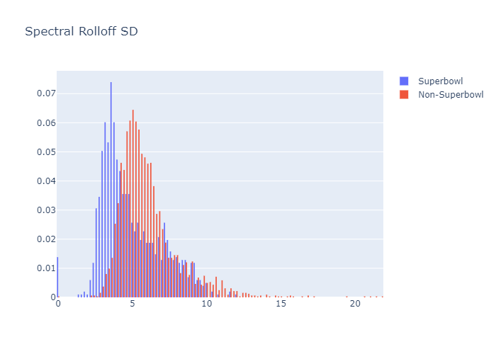
Spectral rolloff is the frequency value that is greater than exactly 85% of the remaining frequency energy of an audio frame. Rolloff standard deviations depict the variety in this value over the duration of the commercials.

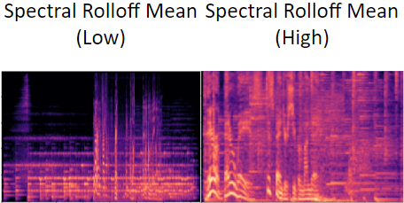
Two spectrograms for commercial with differing spectral rolloff averages are shown. On the left, low spectral rolloff average, right high spectral rolloff average. The corresponding audio files would have a notable average frequency difference, with the left having a lower frequency.

For the video features, instead of all of them being an average over every single frame in a commercial, we instead used a module to detect the scene cuts and used the midpoint frame of each scene. This was mainly due to minimizing the length of computation for each feature. However, the midpoint of each scene should still be quite similar to the rest of the scene, as scene cuts are measured by their difference in pixels, thus each midpoint should act as a good representation for each scene as a whole. As a benefit and drawback to this, the length of each scene is ignored as a potential feature, however their averages can still be found using the number of scenes and the overall length of the given commercial.

For each scene, we used OCR and Face detection to get the average counts of words and faces respectively. We only used these simple versions of these features for a few specific reasons. For OCR, we found that it often was ineffective at effectively finding text in each scene midpoint, namely due to the fact that each non-superbowl commercial had a watermark made out of text, and the OCR implementation didn’t consistently detect it. For Face detection, we found that it required a large amount of computational power for anything more than face detection, such as sentiment analysis and ethnicity detection.

We also found the average Hue, Saturation, and Brightness values for each commercial as well, following the previous Mondrian Complexity analysis we performed in the class. We decided not to use the edge score previously implemented as we felt that it wasn’t likely to have any merit in the model.

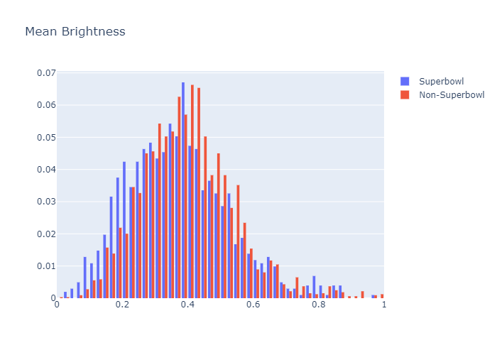
A histogram showing the percentage frequencies of average brightness, categorized. No significant difference between the categories is seen.

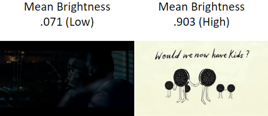
Two frames from 2 separate commercials, with left being low brighness from a superbowl commercial, and right being high brightness from a non-superbowl commercial.

Models and Their Effectiveness

The two models we used were a logistic regression and random forest model. Both used all the numerical features generated, with scaling for each feature.

Logistic Regression			Random Forest
Accuracy (%)			Accuracy (%)
Combined	87.3%		Combined	90.6%
Superbowl	63.4%		Superbowl	69.5%
Other	96%		Other	97.5%
F1 Score:	.727

Our overall accuracies for both models were notably effective, however random forest was more effective than logistic regression. The superbowl accuracies for both were less accurate, thus showing that both models were either overfitted for non-superbowl commercials or had features that were not able to represent any notable differences between the two. The former reason would make the most sense, as there were three times as many non-superbowl commercials as there were superbowl commercials.

Feature Name:	Importance Score:
MFCC 1 SD	-4.125263
Spectral Rolloff Avg	-3.796118
MFCC 1 Avg	1.889190
Spectral Rolloff SD	1.496879
MFCC 2 Avg	1.456543
Length (Seconds)	-0.906488
MFCC 4 Avg	0.901886
MFCC 3 Avg	-0.862177
Spectral Contrast 5 Avg	0.830333
Spectral Contrast 2 SD	0.815055

For the table above, the importance scores were the coefficient values for the scaled logistic regression model, sorted by the absolute values of their coefficients. The random forest model isn’t represented above as it has an inherent issue where measuring feature importance is incredibly difficult.

Looking at the largest importance scores, all of the most important features are audio features, the only exception being length of the commercial. This likely means that the audio features chosen represent the 2 categories of our commercials better than the video features. It is worth mentioning that there were a total of 100 audio features and less than 10 video features.

Summary of Results/Conclusion

We learned a lot about how inherent audio and video aspects vary by Super Bowl status. We learned that Super Bowl commercials tend to have lower brightness, higher spectral rolloff, and a higher spectral contrast. In simpler terms, videos matching this description are darker, are more densely contained in higher frequencies, and display a wider range of frequencies per audio frame. These are real values and can correspond to recognizable recommendations to filmmakers or directors. Many other features beyond these proved distinguishing. Between the 100+ features utilized, there is plenty of room to learn certain combinations that create distinct video personalities.

More meta analysis on celebrity cameos, textual sentiment, or humor could bring about an even better understanding of the differences that make Super Bowl commercials unique. Additional data, including videos from before 2013, commercials from other major televised events, and commercials from other countries could all yield interesting conclusions to serve in conjunction with or as extension of our analysis.